Parent info
Parts you need
Affiliate links — we may earn a small commission
Try this circuit in your browser!
Run the code, press the buttons and watch what happens — before you buy any parts. No account needed.
Open in Simulator →Your classmates took the derivative on paper. You watched yours update in real time.
Imagine this: AP Calculus, derivatives and rates of change. Everyone differentiates f(x) = 3x² and writes f’(x) = 6x. Correct. Abstract.
Your device: an ultrasonic sensor pointed at you. As you walk toward or away from it, the OLED plots your position (the function). Below that, it plots your velocity — the live derivative. Walk fast: the derivative graph spikes. Walk slow: it’s nearly flat. Stand still: derivative = 0. Slow down: the velocity curve slopes toward zero, showing deceleration.
“The derivative of position is velocity. Here it is. In real life.”
That’s what we’re building. For about $22.
What you’ll need
| Part | What it does | Price |
|---|---|---|
| ESP32-S3-DevKitC-1 | Brain — measures distance, computes derivative, graphs both | ~$12 |
| HC-SR04 ultrasonic sensor | Measures distance 2–400cm, ±3mm accuracy | ~$4 |
| OLED display 0.96” | Shows position graph + velocity (derivative) graph | ~$4 |
| Breadboard + jumper wires | Wires it all | ~$5 |
| 1kΩ + 2kΩ resistors | Turn the sensor’s 5V echo signal into a safe 3.3V | ~$1 |
You also need: a clear area (2–3 meters) to walk in front of the sensor.
Total: ~$22 | Time: ~2 hours | Difficulty: ●●●○○
How it works (60 seconds)
The HC-SR04 sends an ultrasonic pulse (40kHz — too high for human ears) and listens for the echo. Time from pulse to echo, divided by 2 (round trip) and multiplied by the speed of sound (343 m/s) = distance.
Distance over time = position function f(t).
The derivative f’(t) = change in position / change in time = velocity.
We calculate this numerically: velocity = (current_distance - previous_distance) / time_interval
The OLED shows both graphs simultaneously: position on top, velocity on the bottom. Calculus becomes visible.
Step 0: Understand the math first
Position, velocity, and acceleration:
| Physical quantity | Calculus term | What it means |
|---|---|---|
| x(t) = distance from sensor | Function | Your position |
| x’(t) = Δx/Δt | First derivative | Your velocity |
| x’’(t) = Δv/Δt | Second derivative | Your acceleration |
Numerical differentiation:
For discrete measurements:
v(t) = [x(t + Δt) - x(t)] / ΔtFor smoother estimates, use centered differences:
v(t) = [x(t + Δt) - x(t - Δt)] / (2Δt)This is the finite difference method — how computers calculate derivatives when you don’t have an analytic formula.
Step 1: Wire it up
Time: ~10 minutes
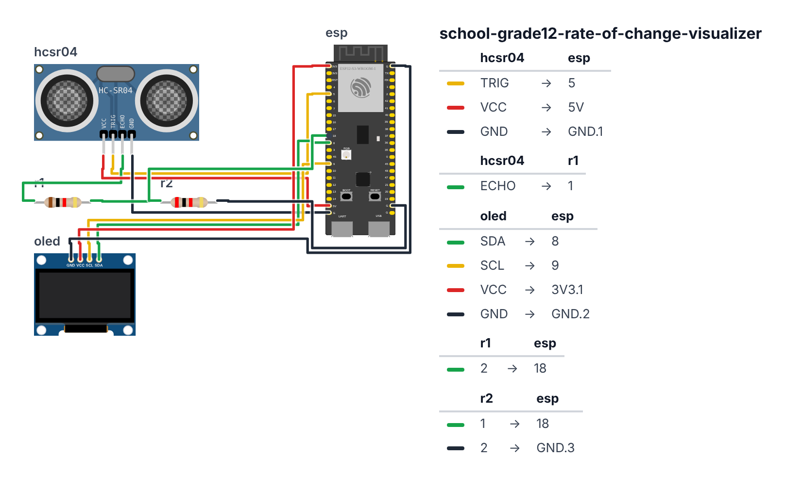
HC-SR04:
- VCC → 5V
- GND → GND
- TRIG → board GPIO 5 (trigger pulse)
- ECHO → 1kΩ resistor → board GPIO 18 (echo return)
- 2kΩ resistor from board GPIO 18 → GND — so the 5V echo signal becomes a safe 3.3V
Note: The HC-SR04 needs 5V, so its ECHO pin also sends back 5V — too much for the ESP32, whose pins only handle 3.3V. The two resistors (1kΩ + 2kΩ) shrink that echo signal to a safe 3.3V before it reaches GPIO 18. Don’t skip them.
OLED: 6. SDA → board GPIO 8 (C6: GPIO 6) 7. SCL → board GPIO 9 (C6: GPIO 7) 8. VCC → 3.3V 9. GND → GND
Step 2: Flash the code
Time: ~20 minutes
Install: Adafruit SSD1306, Adafruit GFX Library
The big picture first. This program turns the ESP32 into a live calculus demonstration device:
- The HC-SR04 ultrasonic sensor measures your distance from it up to 300cm, about 20 times per second.
- Your position over time is f(t) — the function.
- The derivative f’(t) is calculated as
(current position − previous position) / time between readings— the definition of a derivative, done numerically. - Both graphs are drawn simultaneously on the split OLED screen: position on top, velocity (derivative) on the bottom.
- Smoothing blends each new reading with the previous one so sensor noise doesn’t create wild spikes in the derivative.
A program is like a recipe. Copy this entire recipe into Arduino IDE and upload it:
// ========== CHOOSE YOUR BOARD ==========
// Uncomment the line for YOUR board:
#define BOARD_S3    // ESP32-S3-DevKitC-1
//#define BOARD_C6  // ESP32-C6-DevKitC-1
// ========================================

#ifdef BOARD_S3
  #define PIN_SDA    8
  #define PIN_SCL    9
  #define PIN_TRIG   5
  #define PIN_ECHO   18
#endif
#ifdef BOARD_C6
  #define PIN_SDA    6
  #define PIN_SCL    7
  #define PIN_TRIG   5
  #define PIN_ECHO   18
#endif

#include <Wire.h>
#include <Adafruit_GFX.h>
#include <Adafruit_SSD1306.h>

Adafruit_SSD1306 display(128, 64, &Wire, -1);

#define TRIG_PIN PIN_TRIG
#define ECHO_PIN PIN_ECHO

const int GRAPH_WIDTH = 128;
float positionBuf[GRAPH_WIDTH];
float velocityBuf[GRAPH_WIDTH];
int bufferIdx = 0;

float prevPosition = 100.0;
unsigned long prevTime = 0;

float maxPos = 200.0;
float maxVel = 100.0;
float minVel = -100.0;

float measureDistance() {
  digitalWrite(TRIG_PIN, LOW);
  delayMicroseconds(2);
  digitalWrite(TRIG_PIN, HIGH);
  delayMicroseconds(10);
  digitalWrite(TRIG_PIN, LOW);

  long duration = pulseIn(ECHO_PIN, HIGH, 30000);
  if (duration == 0) return -1;

  float distance = (duration / 2.0) * 0.0343;
  return constrain(distance, 2.0, 300.0);
}

float smoothedPos = 100.0;

void drawDualGraph() {
  display.clearDisplay();

  display.drawFastHLine(0, 32, 128, SSD1306_WHITE);

  float maxAbsVel = 10.0;
  for (int i = 0; i < GRAPH_WIDTH; i++) {
    if (abs(velocityBuf[i]) > maxAbsVel) maxAbsVel = abs(velocityBuf[i]);
  }

  display.setTextSize(1);
  display.setCursor(0, 0);
  display.print("x:");
  display.print(smoothedPos, 0);
  display.print("cm");

  for (int x = 0; x < GRAPH_WIDTH; x++) {
    int idx = (bufferIdx + x) % GRAPH_WIDTH;
    if (positionBuf[idx] <= 0) continue;
    int y = map((int)positionBuf[idx], 0, (int)maxPos, 30, 2);
    y = constrain(y, 2, 30);
    display.drawPixel(x, y, SSD1306_WHITE);
  }

  display.setCursor(0, 35);
  float curVel = velocityBuf[(bufferIdx + GRAPH_WIDTH - 1) % GRAPH_WIDTH];
  display.print("v:");
  display.print(curVel, 0);
  display.print("cm/s");

  display.drawFastHLine(0, 48, 128, SSD1306_WHITE);

  for (int x = 0; x < GRAPH_WIDTH; x++) {
    int idx = (bufferIdx + x) % GRAPH_WIDTH;
    int y = map((int)velocityBuf[idx], -(int)maxAbsVel, (int)maxAbsVel, 62, 34);
    y = constrain(y, 34, 62);
    display.drawPixel(x, y, SSD1306_WHITE);
  }

  display.display();
}

void setup() {
  Serial.begin(115200);
  Wire.begin(PIN_SDA, PIN_SCL);
  display.begin(SSD1306_SWITCHCAPVCC, 0x3C);

  pinMode(TRIG_PIN, OUTPUT);
  pinMode(ECHO_PIN, INPUT);

  for (int i = 0; i < GRAPH_WIDTH; i++) {
    positionBuf[i] = 100.0;
    velocityBuf[i] = 0.0;
  }

  prevTime = millis();
  Serial.println("time_ms,position_cm,velocity_cms");
}

void loop() {
  float raw = measureDistance();
  if (raw < 0) { delay(50); return; }

  smoothedPos = 0.7 * smoothedPos + 0.3 * raw;

  unsigned long now = millis();
  float dt = (now - prevTime) / 1000.0;

  float velocity = 0;
  if (dt > 0.01 && prevPosition > 0) {
    velocity = (smoothedPos - prevPosition) / dt;
    velocity = constrain(velocity, -200, 200);
  }

  positionBuf[bufferIdx] = smoothedPos;
  velocityBuf[bufferIdx] = velocity;
  bufferIdx = (bufferIdx + 1) % GRAPH_WIDTH;

  prevPosition = smoothedPos;
  prevTime = now;

  Serial.println(String(now) + "," + String(smoothedPos, 1) + "," + String(velocity, 1));

  drawDualGraph();
  delay(50);
}
Line-by-line: what every line does and why
Lines 1–3: Borrowing ready-made tools
#include <Wire.h>
#include <Adafruit_GFX.h>
#include <Adafruit_SSD1306.h>
#include means “grab this instruction book.” Three books for I2C communication, graphics, and the OLED display.
Lines 5–7: Pin names
#define TRIG_PIN PIN_TRIG
#define ECHO_PIN PIN_ECHO
TRIG (leg 5) is the output pin — the ESP32 sends a pulse here to fire the ultrasonic sensor. ECHO (leg 18) is the input pin — the ESP32 listens here for the returning sound pulse. These two pins are always needed for the HC-SR04.
Lines 9–14: Circular graph buffers
const int GRAPH_WIDTH = 128;
float positionBuf[GRAPH_WIDTH];
float velocityBuf[GRAPH_WIDTH];
int bufferIdx = 0;
GRAPH_WIDTH = 128 matches the OLED’s 128-pixel width — each column of the screen holds one reading. positionBuf and velocityBuf are like scrolling paper tape recorders. bufferIdx tracks which slot gets the next reading. When it reaches 127, it wraps back to 0 — like a clock, the oldest data is overwritten by the newest.
Lines 16–22: Variables for smoothing and physics
float prevPosition = 100.0;
unsigned long prevTime = 0;
float smoothedPos = 100.0;
prevPosition and prevTime remember the last measurement so we can calculate how much position changed since then. smoothedPos is the filtered version of the raw reading — it starts at 100cm as a reasonable default.
Lines 24–35: measureDistance() — the sonar sequence
float measureDistance() {
  digitalWrite(TRIG_PIN, LOW);
  delayMicroseconds(2);
  digitalWrite(TRIG_PIN, HIGH);
  delayMicroseconds(10);
  digitalWrite(TRIG_PIN, LOW);

  long duration = pulseIn(ECHO_PIN, HIGH, 30000);
  if (duration == 0) return -1;

  float distance = (duration / 2.0) * 0.0343;
  return constrain(distance, 2.0, 300.0);
}
The HC-SR04 fires a short ultrasonic burst when TRIG goes HIGH for 10 microseconds. Sound travels out, hits an object, bounces back. The ESP32 waits on the ECHO pin.
pulseIn(ECHO_PIN, HIGH, 30000) measures how long ECHO stays HIGH (in microseconds). 30000 is the timeout — if no echo within 30ms, return 0.
duration / 2.0 converts round-trip time to one-way time (sound went out AND came back). * 0.0343 converts microseconds to centimeters (sound travels 0.0343 cm/µs at room temperature).
constrain(distance, 2.0, 300.0) clips the result to the sensor’s valid range — less than 2cm or more than 300cm would be unreliable.
Lines 37–80: drawDualGraph() — the split screen
display.drawFastHLine(0, 32, 128, SSD1306_WHITE);A horizontal white line at y=32 divides the screen in half. The top half (y=0 to 31) shows position. The bottom half (y=33 to 63) shows velocity.
float maxAbsVel = 10.0;
for (int i = 0; i < GRAPH_WIDTH; i++) {
  if (abs(velocityBuf[i]) > maxAbsVel) maxAbsVel = abs(velocityBuf[i]);
}
Auto-scaling: find the maximum absolute velocity currently in the buffer. The graph will always use the full height no matter how fast or slow you move. This is why the graph adjusts — slow walking fills the full velocity half, fast running also fills the full velocity half.
int idx = (bufferIdx + x) % GRAPH_WIDTH;Circular buffer reading: bufferIdx points to the oldest data (the next slot to be overwritten). Reading from bufferIdx forward wraps around correctly using %. The graph always shows the oldest data on the left and the newest on the right.
int y = map((int)positionBuf[idx], 0, (int)maxPos, 30, 2);map() converts a position in centimeters to a pixel row. Larger distance → lower position on top graph (y closer to 30). Smaller distance → higher on top graph (y closer to 2). This means “close” appears at the top of the position graph.
int y = map((int)velocityBuf[idx], -(int)maxAbsVel, (int)maxAbsVel, 62, 34);For velocity: zero maps to the middle of the bottom half (y=48, the horizontal zero line). Positive velocity maps above zero (moving away). Negative velocity maps below zero (approaching).
Lines 82–104: setup() — the morning routine
for (int i = 0; i < GRAPH_WIDTH; i++) {
  positionBuf[i] = 100.0;
  velocityBuf[i] = 0.0;
}
Pre-fill both buffers with default values. Without this, the graphs would show random garbage on startup.
Lines 106–127: loop() — the derivative in action
smoothedPos = 0.7 * smoothedPos + 0.3 * raw;Exponential smoothing: instead of using the raw distance directly, blend it with the previous smoothed value: 70% old + 30% new. This removes jitter. If the sensor gives a noisy spike, it only affects the result by 30%, not 100%. This is the same technique used in stock market moving averages and audio signal processing.
float dt = (now - prevTime) / 1000.0;
float velocity = (smoothedPos - prevPosition) / dt;
This IS the derivative formula: Δposition / Δtime = velocity. dt is the time gap between measurements in seconds. smoothedPos - prevPosition is how far you moved. Dividing gives speed in cm/s. A positive number means you’re moving away from the sensor; negative means you’re approaching.
bufferIdx = (bufferIdx + 1) % GRAPH_WIDTH;Advance the write position. After slot 127 comes slot 0 again. % is the remainder operator — “wrap around.”
The whole thing in one sentence
Every 50ms, the sensor fires a sound pulse and measures how far you are. The code smooths the reading, calculates how fast your position changed (the derivative), stores both in a circular buffer, and draws the two scrolling graphs side by side.
First thing to try: stand about 100cm from the sensor and hold perfectly still. Both graphs should be flat lines — zero velocity means the derivative of a constant is zero. Now walk slowly toward it: the position line descends, the velocity line goes slightly negative. Walk fast: the velocity line goes very negative. Stop suddenly: the velocity line snaps back to zero.
Check: Upload. Stand 1 meter from the sensor. The position graph should show a roughly flat line at ~100cm. Walk closer — the position line drops, the velocity line goes negative (approaching). Walk back — velocity goes positive (receding).
Step 3: Explore the math physically
Experiments to run:
1. Constant velocity: Walk toward the sensor at a steady speed. Position graph = straight declining line. Velocity graph = flat horizontal line. “Constant velocity = zero acceleration.”
2. Acceleration: Start from a stop, walk steadily faster. Position line curves (parabola-like). Velocity line rises linearly. “Increasing velocity = positive acceleration.”
3. Deceleration: Walk fast, then stop. Velocity graph rises then drops to zero. The moment it drops = inflection point in position graph. “Maximum velocity = inflection point in position function.”
4. Bounce oscillation: Walk toward, stop, walk back — repeat. Position graph oscillates like a sinusoidal. Velocity graph oscillates but shifted 90° (cosine vs. sine). “Velocity of sin(t) = cos(t) — a 90° phase shift.”
Serial data: Export Serial CSV for your report. Paste into Google Sheets. Plot position and velocity on the same chart with two Y-axes.
Presentation tip: Mount the sensor at head height facing the room. Do a live demo — walk toward it while the OLED is projected. Say: “The top graph shows where I am. The bottom shows how fast I’m moving. Right now: walking toward it — position decreasing, velocity negative. As I slow down, watch the velocity line approach zero before position stops changing.”
What just happened
You implemented finite difference differentiation — the numerical method for calculating derivatives from discrete data. The formula v = Δx/Δt is the definition of the derivative, approximated for finite (not infinitesimal) time steps.
Smoothing (0.7 * prev + 0.3 * new) is an exponential moving average — it removes sensor noise by weighting recent values more than old ones. Without this, numerical derivatives amplify noise. This is why signal processing always filters before differentiating.
Curriculum connections:
- AP Calculus AB/BC: Definition of the derivative, rates of change, motion problems
- AP Physics: Kinematics, velocity and acceleration as derivatives
- Common Core Math HSF.IF.B.6: Calculate and interpret the average rate of change of a function over a specified interval
Autonomous vehicles use the same numerical differentiation — GPS position data → velocity estimate → acceleration estimate — to understand their own motion. Your device uses exactly the same algorithm.
Level Up
Second derivative (acceleration): Differentiate the velocity buffer to get acceleration. Add a third graph row. Show that constant velocity → zero acceleration. Sudden stop → spike in acceleration.
Integral: Run the velocity buffer through numerical integration (Riemann sum). The result should match the position measurement. Verify your position by integrating velocity from an initial position.
Predict future position: If velocity is V and acceleration is A, where will the object be in 1 second? Display a predicted cursor on the position graph.
Troubleshooting
| Problem | Fix |
|---|---|
| Distance reads -1 (no echo) | Object too far (>3m) or at a bad angle. Point sensor directly at a flat wall. |
| Graph flickers wildly | Reduce 0.3 smoothing factor to 0.1 for more smoothing. |
| OLED blank | Check SDA=GPIO 8, SCL=GPIO 9 (C6: SDA=GPIO 6, SCL=GPIO 7). Try address 0x3D. |
| Velocity always zero | Check dt calculation. prevTime must be updated each loop. |
| Upload fails | Hold BOOT button while clicking Upload. |